Block calculates numeric solution of a 1st-order nonlinear system with structure according to the picture below - the loop consists of a 1st-order linear system and an isolated hard nonlinearity. As to the type of the nonlinearity, there are four possible options: ideal relay, saturation, relay with dead-zone and relay with hysteresis.
The time interval in which the solution is calculated is specified by Simulink simulation parameters, however, if either NaN or Inf value is reached during the simulation, it is stopped immediately. The block is usually used in combination with the Vector XY Graph for Phase Portraits block that plots the calculated solution in phase plane, but it can also co-operate with other blocks (e.g. Selector or Scope) in order to treat phase trajectories individually.
The block has two vector outputs: y(t) = x1(t) and y'(t) = x2(t) i.e. vectors of horizontal and vertical coordinates of the phase-plane portrait corresponding to different initial conditions.
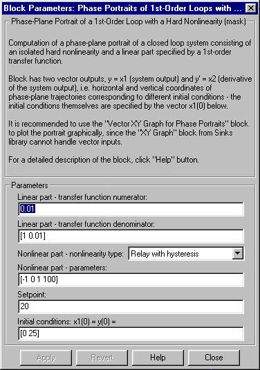
Coefficients of the numerator and the denominator of the transfer function of the linear part of the loop. The block requires two coefficients for the denominator (a vector with two elements) and one coefficient for the numerator.
Dropdown menu for selection of the nonlinearity type. There are following four options:
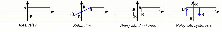
Vector of parameters determining the characteristics and the behaviour of the nonlinearity; the number of the parameters depends on the nonlinearity type. To understand the meaning of these parameters, see the following table:
| Nonlinearity type | Parameters | Parameter definitions |
|---|---|---|
| Ideal relay | [k1 k2] | u = k1 if e < 0, u = k2 if e >= 0 |
| Saturation | [b1 k1 b2 k2] | u = k1 if e <= b1, u = k2 if e >= b2, u = (k2-k1)/(b2-b1)*e + k1 - b1*(k2-k1)/(b2-b1) otherwise |
| Relay with dead-zone | [b1 k1 b2 k2] | u = k1 if e <= b1, u = 0 if b1 < e < b2, u = k2 if e >= b2 |
| Relay with hysteresis | [b1 k1 b2 k2] | u = k1 if e <= b1, u = k1 if b1 < e < b2 a e' > 0, u = k2 if b1 < e < b2 a e' <= 0, u = k2 if e >= b2 |
Desired value (denoted as w in the introductory picture). This value is often equal to zero.
Real vector determining initial points of phase trajectories. Elements of the vector correspond to the x1-coordinates, the x2s are computed so that the points belong to system phase-plane trajectories. The size of the initial conditions vector determines the number of simultaneously running calculations.
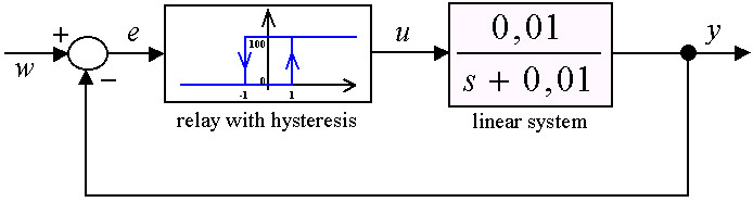
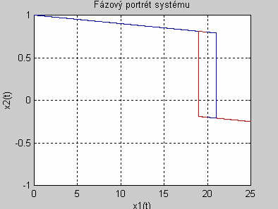
Simulink scheme and phase-plane portrait for above nonlinear loop, initial conditions being x1(0) = 0 and x2(0) = 25. Setpoint w = 20.